

Microsecond Optical Switching. Millisecond Reality.
Budgeting OCS Control Latency, from SDN Orchestration to Device Execution

Optical circuit switches (OCSs) are moving into sub-millisecond reconfiguration. In March 2025, ahead of OFC, iPronics unveiled ONE-32, calling it “the world’s first silicon photonics OCS” and promising reconfiguration in under 300 μs. Microsecond switching has become a selling point for data center products. In September 2026, iPronics announced a $125 million Series B round with NVIDIA participation to support commercial deployment of its optical networking technology for AI data centers.
Faster switching opens up more applications for optical networking. At the 2026 OCP Global Summit, James Burch of Lumotive and Vivek Sarathy of iPronics summarized this shift as “Faster Switching Expands its Use Cases” in Fast switching OCS for AI and Hyperscale Data Centers: Benefits, Technologies and Emerging Applications. As reconfiguration enters the sub-millisecond range, optical connections can follow traffic demand and AI communication phases more frequently, supporting dynamic traffic grooming, topology changes between phases, and finer-grained circuit scheduling. Speed makes uses previously limited by reconfiguration delays worth exploring.
Meanwhile, unified models, interfaces, and multi-vendor orchestration within existing SDN systems have become a major focus of OCS integration. This approach reuses mature network management capabilities. When reconfiguration must keep up with application communication phases, it also requires revisiting the timing assumptions of existing control workflows. In Optically-Accelerated AI Clusters Enabled by Interoperable Multi-Vendor OCSs: Use Cases and Opportunities, Iwan Kartawira of iPronics (a co-lead of the OCP OCS sub-project) and Kazuaki Ueda of KDDI explicitly propose “CPO + OCS + SDN,” placing workload optimization within a joint SDN and OCS architecture. Their multi-vendor control path runs from a gNMI client to a gNMI service and generic YANG datastore, then to vendor APIs. Unified models, controllers, and established management protocols form the backbone of this integration approach.
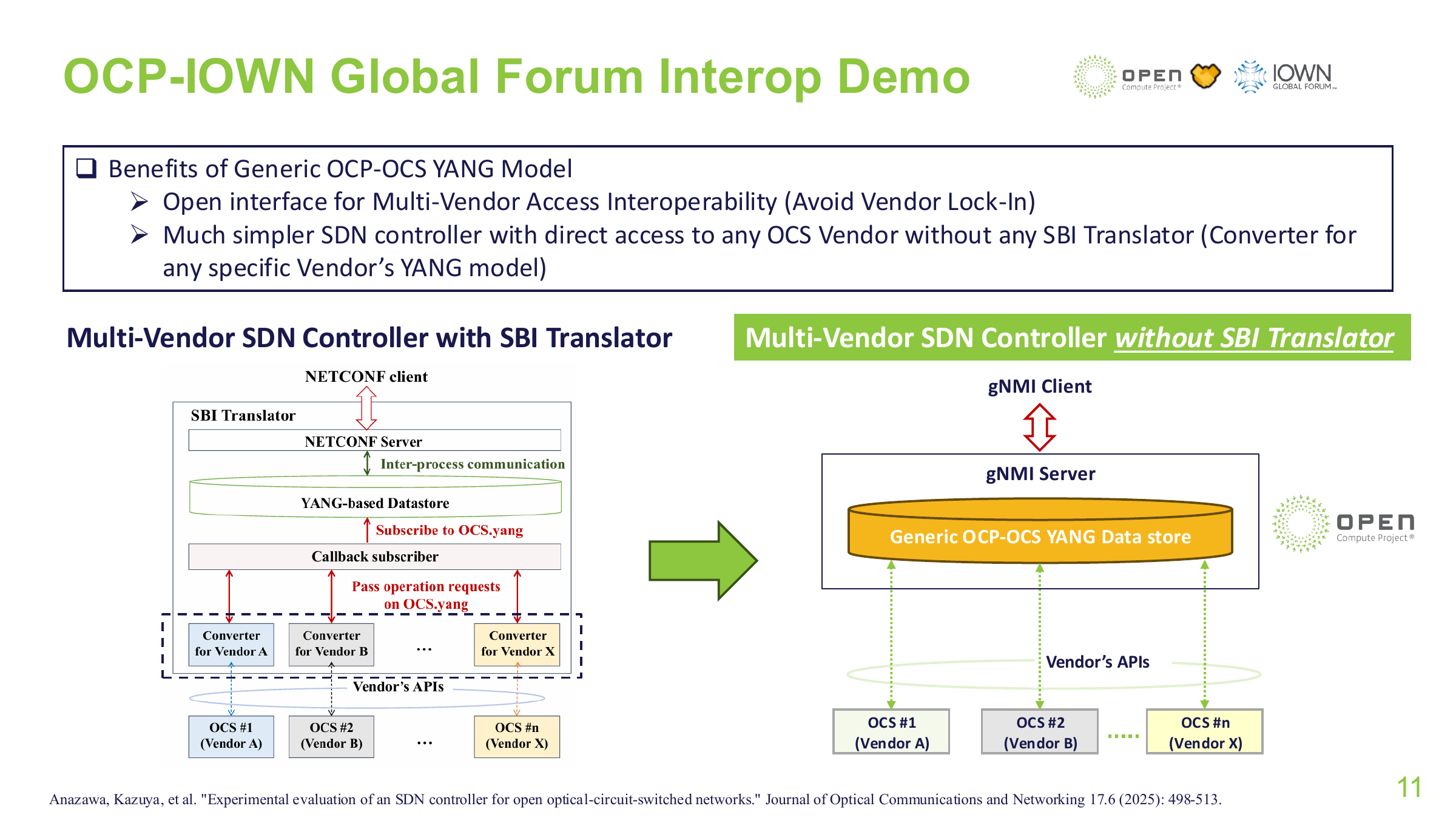
When an OCS reconfigures frequently across communication phases, however, carrying over the full SDN control workflow used for electrical packet networks can make the control path the main limit on reconfiguration speed. In an implementation with controller coordination on every request, the application first contacts the controller, which coordinates resources and calls the device agent (OCS Agent). The device may then invoke local services and SDKs. Global management and vendor adaptation each serve a purpose, but every hop adds communication, validation, scheduling, and queuing.
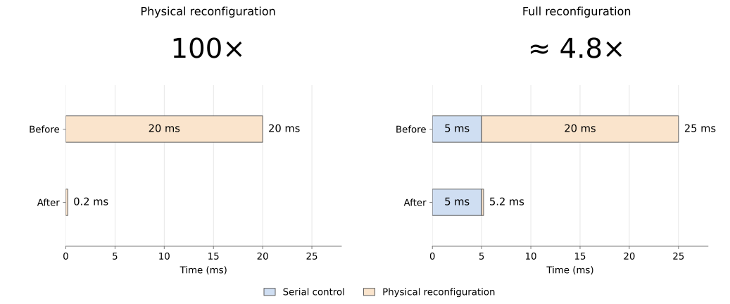
Against the transition from millisecond-scale 3D MEMS to sub-millisecond silicon photonics, consider this calculation: if physical OCS reconfiguration falls from 20 ms to 200 μs while serial control still takes 5 ms, full reconfiguration falls from 25 ms to 5.2 ms. The physical device becomes 100× faster; the full operation becomes only about 4.8× faster. A control architecture organized around slower configuration cycles can consume most of the gains from faster devices when execution must keep up with communication scheduling: the device has reached microseconds, while full reconfiguration remains in milliseconds.
This gap comes from a mismatch between the control architecture and the way fast reconfiguration is used. In a typical SDN packet network, the centralized controller coordinates global resources and configures rules, while switch hardware forwards traffic continuously. This division supports centralized management and fast forwarding: one configuration serves substantial subsequent traffic, so its control cost can be amortized. Individual configuration latency is often less critical.
For applications that reconfigure OCSs with each communication phase, connection setup directly determines when the next phase can transmit. If every reconfiguration follows the full remote coordination and device configuration workflow, the control cost becomes a delay paid before every communication round. Reusing this workflow creates a serious mismatch in timescales for fast OCS switching. In our example, physical reconfiguration has shrunk to 200 μs while the control path still takes 5 ms. Control software now accounts for most of the wait.
The OCP community is advancing unified models, multi-vendor interoperability, and end-to-end metrics. This article asks: when configuration becomes a required step in every communication round, is the existing control architecture still suitable, and how should responsibilities and execution paths change?
A Single Reconfiguration: From Planning to Device Execution
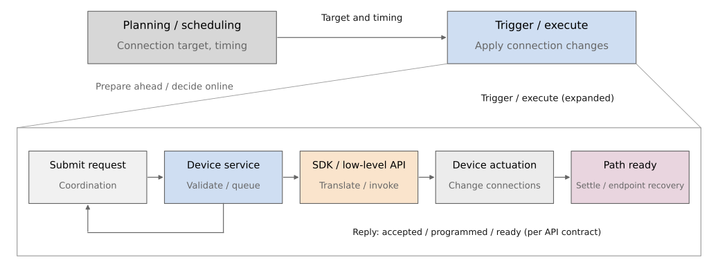
Integrating an OCS into a network starts with deciding which ports to connect, when to change connections, and how to align those changes with application communication phases. The system must then deliver the decision to the device and execute it. These are topology planning and scheduling, followed by triggering and execution. Planning can happen ahead of time; execution is triggered when needed. Predictable targets can be computed in advance, while targets determined by incoming demand require online decisions. Our focus is what happens after the target is known: how much execution remains before the application can use it?
Execution usually begins with a connection request. After any necessary coordination, it reaches the device control service. Device software checks the target and permissions, calls the SDK or low-level API, and translates the port connections into executable device states. OCS implementations differ here.
Google’s Mission Apollo provides a concrete MEMS example: a CPU receives port connection commands, sets micromirror voltages through an FPGA and high-voltage driver boards, and uses camera feedback to adjust the mirrors until the optical path reaches the required state.
In a programmable silicon photonics mesh, the target must also be mapped to internal paths and programmable cell states. translates high-level programs into a graph representation, then solves the mapping onto target photonic hardware.
Interpreting a device’s result requires distinguishing four milestones: request received, programming completed, optical path settled, and application ready. The figure below shows the responsibilities and their dependencies.
The Time Budget: How Much Waiting Remains Beyond the Device?
This framework lets us break down the 5 ms control cost in the opening example. Consider a serial case: the application knows its target and sends a request, the device reconfigures, and the endpoints wait for the path before starting the next communication round. The non-overlapping work intervals are:
T_ready = T_request + T_service + T_apply + T_settle + T_endpointT_request: Request preparation, outbound communication, and any required controller processing.T_service: Device service reception, validation, queuing, and internal handoffs.T_apply: Translating the target into device operations and calling low-level APIs.T_settle: Physical settling still required after those calls.T_endpoint: Remaining endpoint recovery and completion notifications that the application must await.
When work overlaps, use the longest path through the dependency graph. If the SDK already waits for micromirrors to settle, adding the full physical actuation time again would double-count it. Endpoint recovery and device actuation may also run in parallel. This model identifies the work the application must await; inclusive timings from multiple software layers cannot simply be added together.
Temporarily excluding endpoint recovery, let C denote serial control cost and P denote physical reconfiguration. This returns us to T_ready = C + P. The same device speedup produces different full reconfiguration times depending on the control path:
Physical reconfiguration P = 20 ms:
| Serial control C | Total wait C + P | Control share |
|---|---|---|
| 5 ms | 25 ms | 20.0% |
| 500 μs | 20.5 ms | 2.4% |
| 100 μs | 20.1 ms | 0.5% |
Physical reconfiguration P = 200 μs:
| Serial control C | Total wait C + P | Control share |
|---|---|---|
| 5 ms | 5200 μs | 96.2% |
| 500 μs | 700 μs | 71.4% |
| 100 μs | 300 μs | 33.3% |
Both tables calculate control share as C / (C + P). The same control cost accounts for more of the wait as the device becomes faster.
How Does Waiting on the Control Path Add Up to Milliseconds?
Network transmission of a request and reply can first be estimated from their byte sizes. Assume a 1 KiB payload and a further 128 B of encapsulation per direction, crossing two store-and-forward switches and three links. Without retransmissions, serialization in both directions takes about 55 μs at 1 Gb/s or 5.5 μs at 10 Gb/s. Propagation and forwarding are additional costs.
Once the bytes arrive, the request still passes through endpoint software, internal device handoffs, and low-level API calls. Consider a warmed-up connection under low load: the client sends one connection request to the device service; a separate execution process (Worker) calls the low-level API to delete affected old connection entries, waits for the result, then calls it again to install the target entries before replying to the client. One application request thus contains two low-level submissions: deletion and installation. Each submission can batch multiple entries. Drawing on the cost scales of existing packet-switch software stacks gives the hypothetical budget below. It assumes this delete-then-install implementation; it provides neither universal OCS parameters nor measured statistical ranges.
| Part of one synchronous request | Example budget | Work included |
|---|---|---|
| Network transmission of request and reply | 10–80 μs | Serialization, propagation, and switch forwarding; excludes endpoint software |
| Client and device northbound processing | 0.5–1 ms | I/O, encoding/decoding, and dispatch; excludes network transmission |
| Internal device handoffs and non-programming work | 0.5–2 ms | Worker handoffs, validation, queuing, and state processing; excludes low-level calls |
| Deletion and installation in two low-level submissions, combined | 3–4 ms | SDK client, low-level RPC, runtime processing, and waits within calls |
| Total | About 4–7 ms | No separate controller; a Worker; serial deletion and installation |
This example retains the interface processing, separate execution process, and low-level calls common in SDN device software. Even before adding an independent global controller, control already costs about 4–7 ms. Against physical reconfiguration of a few hundred microseconds, this software dominates the wait. Keeping control in step with device speed requires revisiting each stage: which coordination must happen online, which interface capabilities are needed on every request, and which device operations can reduce handoffs or run in parallel?
Architectural Choices: Three Separately Configurable Dimensions
Following a request from the application to the device raises three questions: must a global controller coordinate every operation, which interface admits the request, and how does the device execute it? These form three design dimensions: ① controller participation, ② control interface and protocol, and ③ device execution architecture. We must assess both whether a capability is needed and whether another implementation can provide it within the budget.
| Design dimension | Implementation choices | Main trade-offs |
|---|---|---|
| ① Controller participation | Central coordination on each operation / direct task submission after authorization (fast path) | Boundary between global coordination and local control |
| ② Control interface and protocol | General-purpose RPC / lightweight request–response protocol | Tools and protocol capabilities, processing cost, and maintenance responsibility |
| ③ Device execution architecture | Software: separate Worker / in-process adaptation; Device: individual actuation / batched submission and multichannel control | Isolation and handoffs, configuration transfer efficiency, concurrency, and feedback dependencies |
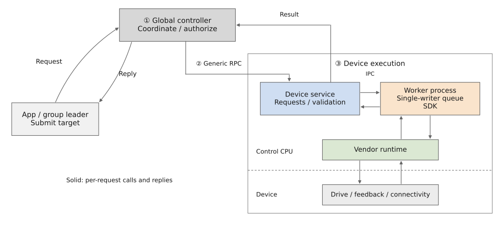
These dimensions can be changed independently. General-purpose RPC can coexist with direct submission within authorized boundaries; a lightweight protocol can still use a separate Worker. We next estimate the scale of work each choice may affect.
① Controller Participation: Central Coordination or Delegated Local Control?
Central coordination has clear value when reconfiguration affects network-wide resources. Google’s Jupiter Evolving, for example, combines OCS topology changes with traffic engineering under centralized SDN. Connection decisions must consider global traffic and topology. Other situations allow a different division. Suppose a communication group exclusively leases a set of ports, and local changes do not affect other jobs. The controller can establish the resource boundary in advance, then let a group representative submit changes directly to the device, matching topology to communication phases within one task. The device still checks permissions, targets, and versions to reject stale writers; the controller still supervises, reclaims resources, and handles recovery. Unified management of global state does not require every authorized local operation to pass through the same remote executor.
This division removes repeated communication, queuing, and processing through the controller while retaining necessary device-side checks. It also requires handling representative failures, lease revocation, and takeover and state reconciliation when request outcomes are unknown. Online arbitration remains necessary where resource boundaries cannot be established in advance. Where they can, that hop can leave the execution path.
For a scale estimate, suppose per-operation coordination adds 100 μs of interaction and 200 μs of processing and queuing, with no overlap. Preauthorization could move about 300 μs off the execution path. For a control budget of only tens of microseconds, this hop alone warrants reconsideration. Actual savings depend on the extra device work needed for direct submission.
② Control Interface and Protocol: General-Purpose RPC or Lightweight Request–Response?
Device management needs rich objects, telemetry, and mature tools. General-purpose RPC can reuse those capabilities. A time-critical reconfiguration may need only a target connection, authorization information, a version, and a completion result. If the general-purpose interface fits the budget, retaining it helps maintenance and integration. If its processing cost is significant, execution can use a narrower interface while YANG continues to describe connections and state and gNMI/gRPC retain management duties.
We explored a lightweight request–response interface using length-prefixed messages and protobuf requests and responses. Persistent TCP connects applications to devices, and Unix domain sockets (UDS) handle internal device communication. This removes some general-purpose RPC processing, while error handling, timeouts, reconnection, and backpressure remain the implementer’s responsibility. The gRPC baseline also reuses connections; the lightweight interface does not provide gNMI’s full protocol capabilities.
With the connection, load, and wire transmission held constant, suppose total protocol processing at both endpoints falls from 200 to 100 μs per complete request–response exchange. One exchange would save about 100 μs, and two serial exchanges about 200 μs.
③ Device Execution Architecture: From Software Handoffs to Parallel Control
③a Software organization determines how many handoffs a request requires. Interface reception, semantic validation, and SDK adaptation are distinct responsibilities. Whether each needs its own process depends on isolation benefits and the time budget. A separate Worker can isolate language runtimes and SDK failures, while adding encoding/decoding, socket operations, thread wakeups, and queuing. In-process adaptation reduces handoffs but needs language and SDK support and broadens the impact of failures. Preserve clear responsibilities, and justify each process boundary by the benefit it provides.
Such handoffs are widely used in packet-switch software, including white-box systems such as SONiC and Stratum. SONiC runs in production data centers at large cloud providers. In its typical architecture,
orchagentexchanges state through Redis withsyncd, which calls vendor SAI/SDK interfaces. This supports modularity and hardware adaptation while adding state conversion, notifications, and process wakeups. A SONiC community proposal for large data center route optimization reports that repeated serial Redis operations add about 500 μs–1 ms per route at scale, and discusses using ZMQ to reduce Redis operations on the critical path. This is the scale reported for that scenario, rather than a fixed cost for all SONiC configurations.
If an internal round trip takes 30 μs and message wrapping and thread dispatch add another 200 μs, merging that handoff could save about 230 μs, assuming negligible additional work for an inline call. Both implementations must coordinate writes to the device so concurrent requests do not overwrite each other.
After reducing software handoffs, device execution still needs inspection: how many operations must a connection target pass through before actual connectivity changes?
③b Device control determines how many steps implement one target. A logical connection may require phase settings for several MZIs or orientation changes for multiple MEMS mirrors on both sides. Combining operations into one command reduces submission cost. Whether the device loads and drives those actuators simultaneously, and how many feedback rounds are needed to settle, are capabilities further down the path. Fewer calls do not establish parallel device execution; simultaneous starts do not establish simultaneous completion.
Apollo illustrates array-level control: the CPU sets MEMS states through an FPGA, high-voltage drivers, and DACs; feedback cameras image each mirror array, allowing the servo system to adjust multiple mirrors.
Multiple tuning elements in silicon photonics can also operate simultaneously, but stages along a connection may depend on one another. A downstream stage may need an upstream stage to settle before it can finish calibration.
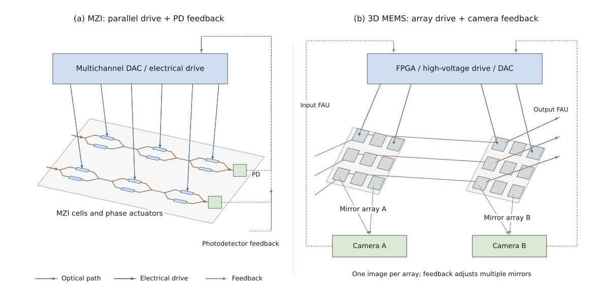
Device execution time can therefore be broken down into command submission, configuration loading, convergence through dependent rounds, and final confirmation. Within each independently parallel round, the slowest relevant channel determines the wait. Dependencies between rounds add further waiting.
Combining the Three Choices into a Candidate Division of Responsibilities
Consider a fast-reconfiguration use case where resources can be allocated in advance, the device can validate authorization, and the SDK supports in-process adaptation. One candidate worth testing has the controller coordinate resources beforehand, then handle authorization, supervision, and reclamation. A group representative submits directly over a lightweight request–response protocol. The device validates and adapts SDK calls in one process, submitting batched targets to the vendor control stack through a single-writer queue. The device applies the target using its own drive concurrency and feedback mechanisms and reports the agreed result. Compared with Figure 4, this combination streamlines all three dimensions, but it is one of many possibilities. Individual choices can also change independently.
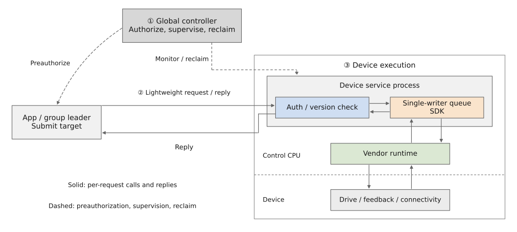
The two architecture diagrams help identify work moved ahead of time, handoffs merged, and device costs that remain. We next introduce the platform and examine which conclusions the evidence supports.
Experimental Platform: Emulating Connection Changes with Intel Tofino
A physical OCS changes optical paths between ports. ReconfigNet-Sim uses an Intel Tofino programmable switch to emulate connection changes by changing which port pairs may forward packets. The P4 pipeline first selects a candidate egress, then checks a permission table for the ingress–egress pair. Only packets permitted by the current connection mapping pass. Updating that table disconnects an old logical connection and enables a new one, providing a repeatable platform for schedulers and control software.
For example, if an application requests a change from A–B to A–C, the device revokes the old forwarding permission and installs the target permission. The application sends only one connection request. The device service may submit deletion of the old permissions to the low-level API, wait for its reply, then submit installation of the target permissions. We call this “separate deletion and installation submissions.” Putting both operations into one low-level request is a “combined submission.” Either submission can contain multiple entries; the count refers to calls from the device service to the low-level API.
The two control paths have comparable responsibilities: an application submits a connection target, a device agent checks and translates it, and a vendor API applies it. In ReconfigNet-Sim, the Agent changes permission entries through a BFRT client and the vendor runtime bf_switchd. This lets us measure software processing, internal handoffs, and device calls, then check their effects with actual packet forwarding.
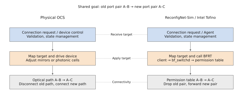
The emulation covers logical connectivity: electrical links stay up, and P4 parses and processes packets. Optical power settling, bit error rate (BER), physical-layer link training, and NIC recovery still require real optical devices. The following measurements were taken on a physical Intel Tofino-1, within the project’s stated boundaries.
Experimental Observations: How Does Reshaping the Control Path Reduce Waiting?
This section fixes the direct-submission fast path described earlier: the client sends connection targets directly to the device service, which retains permission, target, and version checks. The experiments do not compare controller participation modes or measure the cost of passing each request through an independent controller. Within this boundary, we follow the request execution order in Figure 3: ② control interface and protocol, ③a software handoffs within the device service, then ③b low-level API calls. Finally, continuous packet probes check when the new path begins forwarding and how long communication is interrupted during the change.
T_API runs from the client’s request to its successful reply. The SDK programming interval within it, T_SDK, includes SDK client processing, low-level RPC, the vendor runtime, and waits inside the call. It corresponds to the low-level API work within T_apply. We subtract the SDK interval from the API interval for each request before calculating statistics. The remainder includes upper-layer processing and communication; subtracting two p99 values would not produce its p99. Local diagnostics explain costs, while a client on a separate host validates changes to the full path.
Control Interface and Protocol: Streamlining Request–Response Processing
First, consider how a request enters the device. Earlier, we distinguished general device management from time-critical connection execution. Execution primarily needs to carry a target connection, authorization information, a version, and a completion result. We built a lightweight request–response protocol around those requirements, using length prefixes to frame protobuf messages over persistent TCP connections. In the lightweight implementation that retains a separate execution process, internal communication uses the same framing over UDS.
The purpose is to reduce protocol processing and request dispatch in a general-purpose RPC framework. Both interfaces reuse connections, and the lightweight version must still handle errors, timeouts, reconnection, and backpressure. For OCS integration, this is dimension ②: preserve the semantics required for execution while examining how much work the interface’s general capabilities add to every reconfiguration.
After entering the device, the request still passes through validation, translation, and low-level adaptation. These stages contribute to waiting alongside protocol processing. We therefore examine the device service next, then observe their combined effect in the same cross-host comparison.
Device Service: Reducing Handoffs Across Languages and Processes
The external client uses Go, a common choice for network control planes. The device-side interface service that receives network requests also uses Go. Initially, the device retained the vendor’s Python examples and BFRT client, producing a Go interface service plus a Python execution process. The former receives and validates connection targets; the latter translates them into low-level operations. Both run on the device control host and together fulfill the device Agent’s responsibilities.
This division makes existing examples easy to integrate, but each target must cross language and process boundaries. To reduce the software handoffs in ③a, we generated interface code from the public bfruntime.proto and implemented a Go BFRT client. The interface service, validation, and low-level adaptation then run in one process, which continues to connect to the existing vendor runtime, bf_switchd.
Merging processes reduces message passing, thread wakeups, and scheduling. Replacing the client also reduces some request construction and encoding/decoding work. The older Python version and pure-Python protocol library on this platform interpret operations and handle dynamic objects individually; compiled Go code can reduce part of that user-space processing. These costs occur in both the interface service and the SDK client, so changes to software organization can also change the measured SDK programming interval.
Earlier local diagnostics help explain the cost. At about 800 MHz, with deletion and installation still submitted separately, moving from the Go service plus Python execution process to a single Python process, then to a single Go process, reduced the mean interval outside the SDK from about 1003 μs to 667 μs and then 303–307 μs. Further client simplification, a control CPU frequency of about 1.2 GHz, and a different build brought it down to about 140 μs, before combining the low-level submissions.
On the full path between hosts, the lightweight protocol and in-process adaptation together reduced mean API latency from 3777 to 1069 μs. The comparison in Figure 8 uses the same external client and management-network path, with the same performance governor, two fixed control CPU cores, and a frequency of about 1.6 GHz. The northbound protocol, internal handoffs, and BFRT client implementation change together; the result reflects the whole combination.
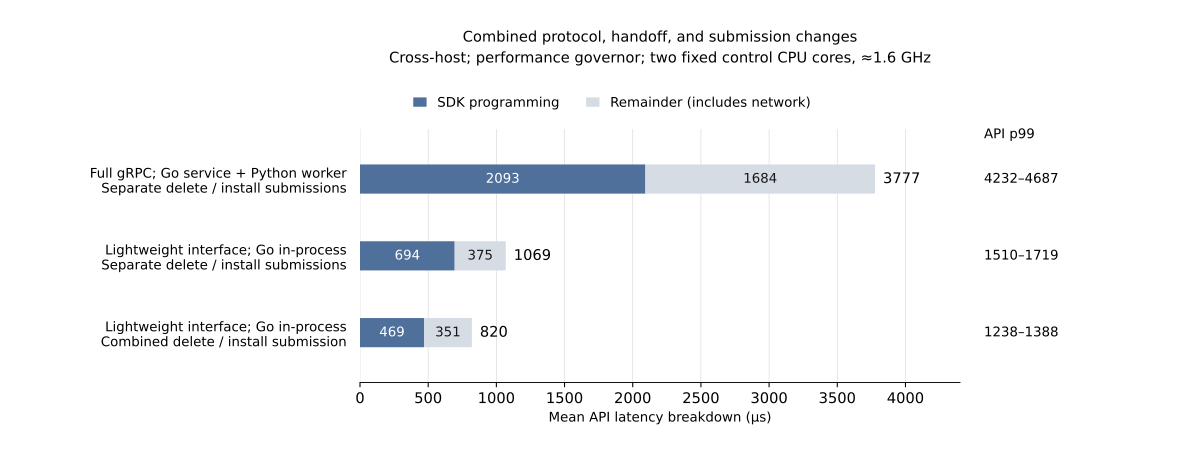
For integration with a physical OCS, this concerns execution within the device service. Target translation, interprocess communication, and request encoding/decoding all enter each reconfiguration’s budget. Evaluating software organization requires examining both the service and its client libraries to determine which work a request still has to await.
Low-Level APIs: Reducing Submissions and Examining the Remaining Wait
Requests now reach the low-level API faster. The next question, from ③b, is: how many serial device operations does one connection target require? The original implementation made separate BFRT submissions to delete old permissions and install target permissions, waiting for bf_switchd after each. Since the service already knows the full target, it can combine both operations into one batched request and remove one low-level API round trip.
For the same Go implementation in Figure 8, mean cross-host API latency falls further from 1069 to 820 μs, while SDK programming falls from 694 to 469 μs. From the original structure to the final candidate, mean API latency falls by about 78%, a speedup of about 4.6×. API p99 values across the final candidate’s repeated runs are 1238–1388 μs.
The local diagnostics in Figure 9 explain the remaining cost. With work outside the SDK already reduced to about 140 μs, combining the submissions leaves about 491–496 μs in the SDK and 632–634 μs in the full API, so the device API path accounts for nearly 78%. This share belongs to the local diagnostic configuration. In the full cross-host candidate, the mean SDK interval is about 469 μs, or 57% of API latency, with about 351 μs remaining. The remainder’s p99 is 492–527 μs.
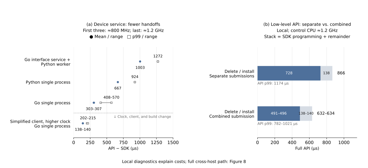
As upper-layer protocol processing and software handoffs shrink, the device API path becomes the largest individual source of waiting. For a physical OCS, further improvement requires device vendors and integrators to optimize control interfaces and runtimes together. Integrators can reduce target translation, request wrapping, and repeated submissions. Vendors need to examine how the runtime receives targets, advances device execution, and reports completion. Whether the system can promptly use faster switching also depends on this control path.
Here, combining requests reduced the number of API steps. For a physical OCS, support for complete connection targets and batch operations determines how many round trips the system pays for. Internal parallelism and the point at which connectivity becomes usable require further checks of device capabilities and completion semantics.
After control requests become faster, when does forwarding actually switch? Separate from the API timings, continuous packet probes measure the time from a request to the first reply over the new path (T_visible) and the blackout between the last reply over the old path and the first over the new one. The first metric shows when the target connection becomes visible to traffic; the second shows how long communication is interrupted.
| Data-plane observation (p99) | Original multiprocess path; separate deletion and installation | Go in-process adaptation; separate deletion and installation | Go in-process adaptation; combined submission |
|---|---|---|---|
Request to first reply over the new path, T_visible | 4000 μs | 1695 μs | 1539 μs |
| Switching blackout | 3113 μs | 1460 μs | 1180 μs |
Within this set of observations, new-path visibility p99 improves by about 61.5%, and blackout p99 by about 62.1%. The control-path changes also improve actual forwarding transitions. The measured probe interval has a p99 of 49–58 μs; observations include probing and receive scheduling. Even the improved p99 cannot guarantee that every transition meets an application’s budget.
These experiments validate changes to the control interface, device service, and low-level submissions. A physical OCS still requires optical settling and endpoint recovery measurements to check the full application-readiness budget.
From Control Budgets to System Design: Recommendations for Industry
Design fast OCS systems by working backward from the application’s waiting-time budget to control responsibilities, interfaces, and device execution. The changes above show that control software determines how much of the device’s speed reaches the application. System integrators, device vendors, and standards communities need to make this time budget concrete in the interfaces and implementations they own.
Organize Execution Around the Application Budget
Use the application’s deadline and the facts that establish readiness as inputs to control architecture. Infrequent topology changes can amortize configuration costs. Reconfiguration at every communication phase incurs those costs before each round. The latter needs execution organized around its budget: where resources can be assigned ahead of time, the controller authorizes and coordinates first, then tasks submit directly within that authorization. The device retains online permission, version, and target checks. Along the three design dimensions, reduce protocol processing, software handoffs, and device operations, and move work that can be completed early away from the trigger.
| Control budget | Target determined when the request arrives | Target can be prepared ahead of time |
|---|---|---|
| Relatively loose, for example several ms | Prioritize general management and isolation, then verify full-path latency | Prepare ahead when the benefits justify the preparation cost |
| Tight, for example tens to hundreds of μs | Streamline online coordination, protocol processing, and handoffs; inspect SDK costs and tail latency | Generate, translate, and load configurations early; select and activate at execution time, with device support |
Turn this table into an explicit division of work. Integrators should list the coordination, validation, translation, loading, and feedback still performed on each request, and explain why each must happen online. Targets for known communication phases can be generated in advance; necessary arbitration for conflicting shared resources still belongs in the budget. The controller continues to own global resource decisions, authorization, supervision, and reclamation. The fast path shortens execution for operations already permitted.
Software-Path Latency Limits: Account for the Work Behind a Microsecond Budget
Estimate software-path limits from required work and dependencies, and check implementations using full-path tail latency. The local software interval fell from about 300 μs to about 140 μs above, showing that implementation and operating conditions still offer room for improvement. Those measurements describe the tested configurations; they do not establish a fixed limit for general-purpose CPUs.
Microsecond communication provides a reference point: eRPC reports a median RPC latency of about 2.3 μs for 32 B messages between two nodes under the same top-of-rack switch on a CX5 Ethernet platform. Taking 20 μs as a p99 budget to be validated for the whole software path means accounting for parsing, validation, translation, scheduling, and necessary handoffs together. The 2.3 μs median illustrates the scale of communication cost; meeting a 20 μs p99 across the control path remains to be demonstrated.
Start by reducing repeated parsing and memory allocation, reusing completed target translations, and shortening thread and process handoffs. For parsing, local validation, and state transitions that must still run at trigger time and have stable semantics, evaluate moving execution into the device or FPGA, leaving policy and exception handling on the control CPU. Choose acceleration targets from the critical path, then verify benefits through complete calls, state consistency, and recovery. Across SDK, runtime, and device boundaries, continue tracing device calls and completion mechanisms. Sato’s optical switching tutorial offers further reading.
Device Vendors Should Deliver Control-Path Performance as a Product Capability
Report latency from receiving a connection target to programming completion and optical readiness alongside device switching specifications. In the cross-host candidate, the SDK interval still represents about 57% of mean API latency, including the client, low-level RPC, vendor runtime, and waits inside calls. After upper-layer simplification, optimization must continue into the device API path. Vendors and integrators should jointly establish how many serial calls a complete target needs, what each call does, and which waits can be combined or removed.
Device interfaces should accept complete connection targets or batch operations to reduce per-item host submissions and waits, while providing explicit completion notifications and necessary state readback. Vendors should also document configuration loading bandwidth, actuator concurrency, and feedback dependencies so integrators can determine the steps needed to apply a target. A successful reply must establish a clear fact: request reception, programming completion, and optical settling each permit different subsequent actions.
For predictable communication phases, split configuration preparation and activation into two interface stages. Generate and load candidate states ahead of time, then activate them through a short command, local event, or scheduled trigger. Define candidate-state capacity, cancellation, and invalidation rules; scheduled activation also needs clock-offset and trigger-accuracy specifications. Preloading moves configuration transfer before the trigger, while device actuation and settling still need a budget. Vendors should implement and validate these capabilities so applications can use them.
Include Timing and Completion Semantics in Interoperability Requirements
Common models and interfaces should come with common timing metrics, completion semantics, and acceptance methods. OCP materials already call for end-to-end metrics and shared service semantics. Communities such as OCP and ODCC should turn those goals into comparable, verifiable interface requirements.
Following Figure 3, specifications should distinguish request reception, programming completion, optical settling, and application readiness, with defined start and end points for each measurement. The device reports programming and optical state; the system checks endpoint recovery and actual communication conditions to reach T_ready. Completion notifications, status queries, and result confirmation after timeouts should be defined around those facts.
Performance reports should state the size of a connection update, load, concurrency, warmup and configuration preparation conditions, and the full path’s mean and tail latency. This lets different protocols, runtimes, and devices be compared at the same endpoint and gives schedulers a basis for arranging the next communication phase. Measuring API replies, the first reply over the new path, and blackout separately above serves exactly this purpose.
Return to the opening example: physical reconfiguration can fall from 20 ms to 200 μs while 5 ms of control leaves the full wait in milliseconds. Faster devices must drive changes in control responsibilities, software paths, and device interfaces, with acceptance based on the full application-readiness budget. Applications can use the speed of improved devices only when this whole path becomes faster.
References and Reading Notes
Core research
- Mission Apollo: Landing Optical Circuit Switching at Datacenter Scale, Section 4.1, Figures 5 and 8a: CPU, FPGA, high-voltage drive, and MEMS feedback control.
- Jupiter Evolving: Transforming Google’s Datacenter Network via Optical Circuit Switches and Software-Defined Networking, SIGCOMM 2022: a production example of centralized SDN, traffic engineering, and topology engineering.
- : A Programming Language for Silicon Photonics and its public compiler: program compilation and hardware mapping.
- Anuj Kalia, Michael Kaminsky, David G. Andersen, Datacenter RPCs can be General and Fast, NSDI 2019, Section 6.1 and Table 2: median latency of 32 B RPCs on different platforms.
- K. Sato, Optical switching will innovate intra data center networks, JOCN 16(1), A1–A23 (2024): further reading on optical switching architectures.
Vendor and OCP community materials
- iPronics ONE-32 announcement, 2025-03-31: the vendor’s <300 μs reconfiguration specification.
- iPronics Series B announcement, 2026-09-02: $125 million, with NVIDIA participation.
- Fast switching OCS for AI and Hyperscale Data Centers: Benefits, Technologies and Emerging Applications, James Burch, Vivek Sarathy, 2026 OCP Global Summit: fast OCS use cases, end-to-end metrics, and coordination requirements.
- Optically-Accelerated AI Clusters Enabled by Interoperable Multi-Vendor OCSs: Use Cases and Opportunities, Iwan Kartawira, Kazuaki Ueda, with Kazuya Anazawa, 2026 OCP Global Summit: CPO + OCS + SDN, workload optimization, and multi-vendor control.
- Zero-Touch OCS Fabrics for AI Scale-Out Infrastructure at Hyperscale, Kannan Raj, Michael DeMerchant: common models, service semantics, path proof, and closed-loop validation.
- OCP Optical Circuit Switching.
Switch software architectures
- SONiC Architecture, the foundation overview, route performance discussions, and the large data center route optimization proposal: production use, software handoffs, and latency scales in specific scenarios.
- Stratum Component Overview: the layers from P4Runtime/gNMI through switch and chip abstractions to SDKs.
Specifications
- RFC 7950: YANG 1.1, Sections 1 and 4.
- gNMI Specification, Sections 3.4.2 and 3.4.3: Set replies and transaction semantics.
Citing Us
Please cite this blog post if you found it helpful. For discussion, contact wuchangbo@sii.edu.cn
@misc{wu2026ocscontrolarch,
  title = {{Microsecond Optical Switching. Millisecond Reality.}},
  author = {Wu, Changbo and Yu, Zhuolong},
  year = {2026},
  month = oct,
  howpublished = {ReconfigNet-Sim Blog},
  url = {https://zer0-nu1l.github.io/ReconfigNet-Sim/en/posts/ocs-control-arch/}
}